An Introduction to the Electronic Structure of Atoms and Molecules
Professor of Chemistry / McMaster University / Hamilton, Ontario
An Introduction to the Electronic Structure of Atoms and MoleculesProfessor of Chemistry / McMaster University / Hamilton, Ontario
|
In quantum mechanics, Newton's familiar equations of motion are replaced by Schrödinger's equation. We shall not discuss this equation in any detail, nor indeed even write it down, but one important aspect of it must be mentioned. When Newton's laws of motion are applied to a system, we obtain both the energy and an equation of motion. The equation of motion allows us to calculate the position or coordinates of the system at any instant of time. However, when Schrödinger's equation is solved for a given system we obtain the energy directly, but not the probability distribution functionCthe function which contains the information regarding the position of the particle. Instead, the solution of Schrödinger's equation gives only the amplitude of the probability distribution function along with the energy. The probability distribution itself is obtained by squaring the probability amplitude. (Click here for note.) Thus for every allowed value of the energy, we obtain one or more (the energy value may be degenerate) probability amplitudes.
The probability amplitudes are functions only of the positional coordinates of the system and are generally denoted by the Greek letter y (psi). For a bound system the amplitudes as well as the energies are determined by one or more quantum numbers. Thus for every En we have one or more yn's and by squaring the yn's we may obtain the corresponding Pn's.
Let us look at the forms of the amplitude functions for the simple
system of an electron confined to motion on a line. For any system, y
is simply some mathematical function of the positional coordinates. In
the present problem which involves only a single coordinate x, the
amplitude functions may be plotted versus the x-coordinate in the
form of a graph. The functions yn
are particularly simple in this case as they are sin functions.
|
|
|
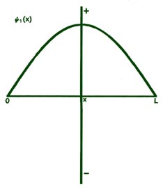
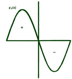


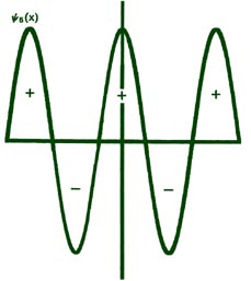
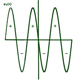
Fig. 2-8. The first six probability amplitudes yn(x) for an electron moving on a line of length L. Note the yn(x) may be negative in sign for certain values of x. The yn(x) are squared to obtain the probability distrubrition functions Pn(x), which are, therefore, positive for all values of x. Wherever yn(x) crosses the x-axis and changes sign, a node appears in the corresponding Pn(x).
Each of these graphs, when squared, yields the corresponding Pn
curves shown previously. When n = 1,
|
|
|
|
|
|
|
|
|
|
As illustrated previously in Fig.
2-4, the value of yn2(x)
or Pn(x) multiplied by Dx,
yn2(x)Dx,
or Pn(x)Dx,
is the probability that the electron will be found in some particular small
segment of the line Dx. The constant
factor of ![]() which appears in every yn(x)
is to assure that when the value of yn2(x)Dx
is summed over each of the small segments Dx,
the final value will equal unity. This implies that the probability that
the electron is somewhere on the line is unity, i.e., a certainty. Thus
the probability that the electron is in any one of the small segments Dx
(the value of yn2(x)Dx
or
Pn(x)Dx
evaluated at a value of x between 0 and L) is a fraction
of unity, i.e., a probability less than one. (Click
here for note.)
which appears in every yn(x)
is to assure that when the value of yn2(x)Dx
is summed over each of the small segments Dx,
the final value will equal unity. This implies that the probability that
the electron is somewhere on the line is unity, i.e., a certainty. Thus
the probability that the electron is in any one of the small segments Dx
(the value of yn2(x)Dx
or
Pn(x)Dx
evaluated at a value of x between 0 and L) is a fraction
of unity, i.e., a probability less than one. (Click
here for note.)
Each yn must necessarily go to zero at each end of the line, since the probability of the electron not being on the line is zero. This is a physical condition which places a mathematical restraint on the yn . Thus the only acceptable yn 's are those which go to zero at each end of the line. A solution of the form shown in Fig. 2-9 is, therefore, not an acceptable one. Since there is but a single value of the energy for each of the possible yn functions, it is clear that only certain discrete values of the energy will be allowed. The physical restraint of confining the motion to a finite length of line results in the quantization of the energy. Indeed, if the line is made infinitely long (the electron is then free and no longer bound), solutions for any value of n, integer or non-integer, are possible; correspondingly, all energies are permissible. Thus only the energies of bound systems are quantized.
 |
Fig. 2-9. An unacceptable form for yn(x). |
|
|
|
A yn does not represent the trajectory or path followed by an electron in space. We have seen that the most we can say about the position of an electron is given by the probability function yn2. We do, however, refer to the wavelengths of electrons, neutrons, etc. But we must remember that the wavelengths refer only to a property of the amplitude functions and not to the motion of the particle itself.
A number of interesting properties can be related
to the idea of the wavelengths associated with the wave functions or probability
amplitude functions. The wavelengths for our simple system are given by
l
= 2L/n. Can we identify these wavelengths with the wavelengths
which de Broglie postulated for matter waves and which obeyed the relationship:
|
|
 |
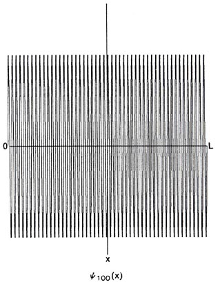
It is clear that as n increases, l becomes much less than L. For n = 100, y100and P100 would appear as in Fig. 2-10. When L>>ln, the nodes in Pn are so close together that the function appears to be a continuous function of x. No experiment could in fact detect nodes which are so closely spaced, and any observation of the position of the electron would yield a result for P100 similar to that obtained in the classical case. This is a general result. When l is smaller than the important physical dimensions of the system, quantum effects disappear and the system behaves in a classical fashion. This will always be true when the system possesses a large amount of energy, i.e, a high n value. When, however, l is comparable to the physical dimensions of the system, quantum effects predominate.

Let us check to see whether or not quantum effects
will be evident for electrons bound to nuclei to form atoms. A typical
velocity of an electron bound to an atom is of the order of magnitude of
109 cm/sec. Thus:
 |
We can also determine the wavelength associated with the
motion of the mass of 1 g moving on a line 1 m in length with a velocity
of, say, 1 cm/sec:
 |
 |
 |
 |
 |